Write a time-series database engine from scratch
This blog post walks you through how to implement a time-series database engine based on what I’ve learned from my experience of writing a lightweight one from scratch.
While it is written in Go, it mostly covers language-agnostic.
Motivation
I’ve been working on a couple of tools that handle a tremendous amount of time-series data. One of them, Ali, is a load testing tool that can plot metrics in real-time on the client side. It requires a certain query performance while the results like latency and any other measurements are being written endlessly for each request. In other words, it’s kind of like making a push monitoring system with simple query feature on a single host.
It was simply appending data points to a variable length array on the heap in previous implementation, which naturally led to the problem of increasing memory usage over time:
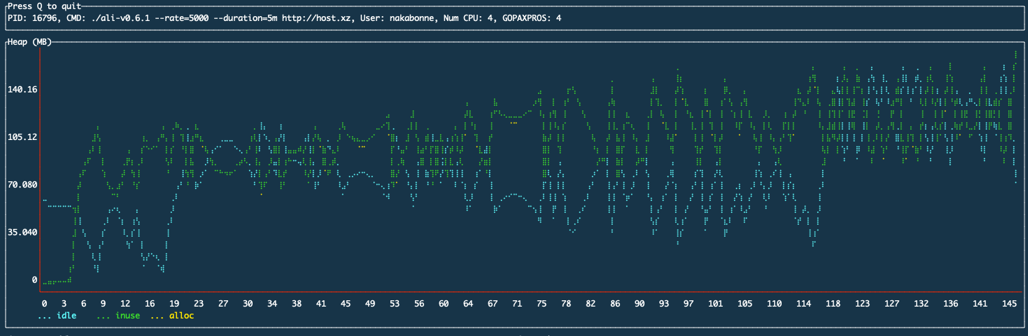
Ali’s heap usage measured by nakabonne/gosivy
I little poked around a storage engine that could be used as a library from the Go program to address this issue.
Characteristics of time-series data
We first need to understand time series data to sort out the problem that needs to be solved,
Time series data is a collection of multiple values with a time stamp. It is usually used to observe data as it changes over time. Each one is called a data point, and is often represented as a tuple with a timestamp and a value. This time series data has the characteristics as:
Tremendous amount of data
Due to the nature of time series data, a single data point is rarely meaningful, and it is only when a large amount of data is collected that it becomes effective. It’s not uncommon in the financial industry for data capture requirements to exceed 1000000/s, as the data is often written over a short period of time.
In Ali’s use case, the request rate specified by the user is directly related to the write performance requirement (although basically the upper limit of the number of file descriptors is the bottleneck).
To deal with this, we need to focus on optimizing the writing process anyway. We also need to do something to minimize the disk space consumed as much as possible.
Append-only
Every data point is immutable. Also, it typically performs delete operations in batches on less recent data, not specifying a specific data point.
Ordered by time
It can be considered as already being indexed by time as the data is stored sorted by timestamps. With it you can build up indexes without any overhead.
Accessed in bulk
When reading out, it’s mostly retrieves multiple data points with consecutive timestamps by specifying a time period. You can improve the locality when reading by focusing on this.
Most recent first
In many use cases, we tend to read and use recent data points. This is likely to affect the choice of cache algorithm.
High cardinality
Time series data tends to have a higher cardinality. This is especially true in the context of system monitoring, for example. In the age of cloud natives, we are getting more opportunities to monitor environments with dynamically changing hosts and networks, etc.
In that sense, there are few kind of metrics that are exactly the same; creating a file for each metric will cause various kinds of problems such as inode limitations.
Existing Solution
In general, we found that time series data is write-heavy, and there are many opportunities to read/write data sequentially within a time range.
Google’s LevelDB is well known as a key-value storage engine, and a couple of implementations in Go have been published. This LevelDB is implemented based on LSM trees, which only writes sequentially to the tails; it works well with appended-only time series data. What it’s sorted by key also makes it suitable for time-series data that is timestamp-based. In fact, the early storage engines of Prometheus and InfluxDB were also based on LevelDB.
However, there are a couple of waste things.As we will see later, time series data is monotonous and can be encoded to a smaller size by taking advantage of this characteristic. Since we deal with time series data which is huge in quantity, we would like to leverage this.
Also, because all data points are immutable and no update process is required, all writes can be done sequentially. Despite this, I was a little concerned about the Write amplification that occurs when merging SSTables and so on.
tstorage
So, I settled on writing a database engine library called tstorage myself.

It is a lightweight engine that uses local disks and is implemented entirely in pure Go.
This post covers how I implemented this, along with an explanation of the knowledge I needed to create it.
What is a database engine?
A typical DBMS handles requests from clients and controls communication between nodes for clustering. It also parses queries, makes execution plans, and reads/writes data from/to disk based on those plans. A database engine is a component that performs only the last read/write part. This is the part of the Storage Engine in the figure below.
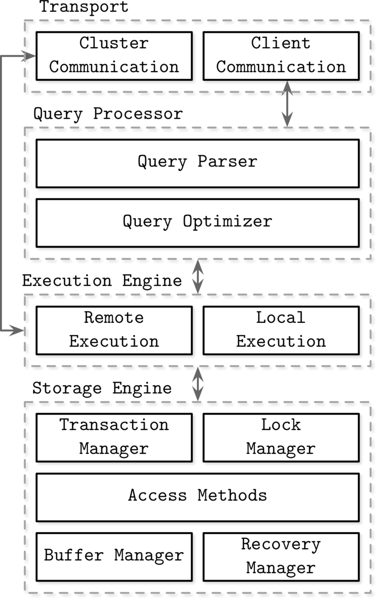
Database Internals, Alex Petrov, 2019, Chapter1, Figure 1-1. Architecure of database management system
It abstracts the data structure on disk/memory and provides API to Execution Engine in this figure. In addition, it also provides transaction and recovery functions.
Data Model
Based on these characteristics, tstorage adopts a linear data model structure that partitions data points by time. Each partition acts as a fully independent database containing all data points for its time range.
  │                 │
Read              Write
  │                 │
  │                 V
  │      ┌───────────────────┐ max: 1600010800
  ├─────>   Memory Partition
  │      └───────────────────┘ min: 1600007201
  │
  │      ┌───────────────────┐ max: 1600007200
  ├─────>   Memory Partition
  │      └───────────────────┘ min: 1600003601
  │
  │      ┌───────────────────┐ max: 1600003600
  └─────>   Disk Partition
         └───────────────────┘ min: 1600000000
Slightly influenced by LSM-trees, Prometheus' V3 storage also uses a model that is quite close.
Only the Head and the next partition are on the heap and are writable. This is called a memory partition. In memory partitions, data is appended to the end of the Write Ahead Log before writing to prevent data loss (this can be turned off if you don’t need such durability).
Older partitions get written to a single file on the disk. This is called a disk partition and is read-only. Files written to disk are transparently cached through the kernel by mmap(2), which will be explained later.
You can set a period of time for the partition, after which a new memory partition will be automatically added to the Head and the old one will be flushed to disk.
This model has a number of advantages. First, partitions outside the specified range can be completely ignored when reading. This idea of narrowing down the search range as much as possible is inspired by the Bloom filter used in LevelDB. Also, since the latest data points are cached in the heap, most reads will be fast.
Besides, because tstorage is designed to write one partition to one file:
- All write operations can be append-only without any Write amplification occurring as it only writes to one file sequentially
- The number of files does not depend on the cardinality (number of metric types)
- It improves locality because reads operations often specify a time period and acquire adjacent data points as mentioned above
The following sections describe the key points in each partition’s implementations.
Memory Partition
Data point list
A list of data points is represented as an array on the heap (technically, it’s kind of like a pointer list to a base array called Slice in Go). This is a list with an unlimited number of data points to be written, so at first glance, Linked-list may seem to be the best choice, as it allows adding elements with O(1). However, arrays whose elements are lined up next to each other in RAM benefit from the spatial locality of cache memory. Also, since the time series data is always pre-sorted, classical search algorithms such as binary search can be easily implemented.
Out-of-order data points
What data points get out-of-order in real-world applications is not uncommon because of network latency or clock synchronization issues. This should be taken into account when writing, and the data points in the partition should always be kept sorted.
However, note that we need to apply an exclusive lock each time we write to them as we are managing data points as arrays. We have to think a cool way to ingest them so that we do not have to extend this lock time to accommodate unordered data points.
Unordered data points can be divided into two cases: first, they are unordered within the range of the partition you are trying to write to. The second case is that the data point is outside of the range of the partition you tried to write to in the first place.
If the written data points correspond to the first case, we will first buffer the data points in a separate array in out-of-order. Then, at the time of flushing to disk, the data points get merged with the data points in the memory partition and re-sorted.
In the data model section, I mentioned that only the Head and its next partition are on the heap, in order to accommodate the second case: soon after a new partition is added to the Head, data points crossing partitions may be written. This is for addressing the second case. By keeping the two most recent partitions writable, we avoid these being discarded.
Write Ahead Log (WAL)
Since memory partitions use volatile storage, there is a possibility of data loss due to sudden crash or power shortage. To deal with this, the memory partition first writes the operation log to the Write Ahead Log (WAL). In the event of a crash, you can recover by executing the operations written from the beginning to the end of the log.
In the case of a database engine that supports on-disk data update operations, WAL has to hold very low-level operations; to fully restore the update process, it is necessary to store exactly which bytes in which disk block were changed, etc.
However, time-series data is append-only, and tstorage makes all disk partitions read-only. It needs to append only high-level information about what data points have been written to the memory partition, so it can recover them with a simple disk-independent format.
Disk Partition
The fastest way to understand disk partitions is to have a look at the macro layout on the file system.
As shown below, it uses one directory per partition, with metadata and the actual compressed data underneath. This is a simplified version of the Prometheus layout, so you may have seen a similar structure before.
$ tree ./data
./data
├── p-1600000001-1600003600
│   ├── data
│   └── meta.json
├── p-1600003601-1600007200
│   ├── data
│   └── meta.json
└── p-1600007201-1600010800
    ├── data
    └── meta.json
I will describe the implementation points in the order of data -> metadata.
Memory-mapped data
As mentioned above, all data points in a partition are written to a single file. tstorage adopts the following format.
    ┌───────────────────────────┐
    │    Metric-1    │ Metric-2 │
    │───────────────────────────│
    │ Metric-3 │                │
    │──────────┘                │
    │          Metric-4         │
    │───────────────────────────│
    │   Metric-5  │   Metric-6  │
    │───────────────────────────│
    │         Metric-7      │   │
    │───────────────────────┘   │
    │         Metric-8          │
    │───────────────────────────│
    │Metric-9│     Metric-10    │
    └───────────────────────────┘
             File format
Metric-1 ~ Metric-10 represent the data point list of metrics respectively.
Recall the characteristics of time series data. Data points were immutable, and mostly, metrics were obtained in bulk by specifying a range. Therefore, we can improve locality by grouping data points by metric.
This file is cached transparently through the kernel in mmap(2). This allows us to cache the file without copying it to user space. This works quite well since my original motivation was to solve the problem of Ali eating up the heap over time.
The memory-mapped file can be accessed by the Go program as []bytes, just like a string of bytes on the heap.
type diskPartition struct {
	// file descriptor of data file
	f *os.File
	// memory-mapped file backed by f
	mappedFile []byte
Now, how do we search for this self-contained byte sequence? It would be easy to copy it onto the heap and decode it into a data structure in the Go program, but that would defeat the purpose of memory mapping. Somehow, we need an index structure to access the encoded data efficiently. The metadata introduced next is used for this purpose.
Metadata
The content of the metadata looks like this. A partition has only one metadata, that’s why the JSON format was adopted, which is somewhat redundant but easy to handle programmatically.
$ cat ./data/p-1600000001-1600003600/meta.json
{
  "minTimestamp": 1600000001,
  "maxTimestamp": 1600003600,
  "numDataPoints": 7200,
  "metrics": {
    "metric-1": {
      "name": "metric-1",
      "offset": 0,
      "minTimestamp": 1600000001,
      "maxTimestamp": 1600003600,
      "numDataPoints": 3600
    },
    "metric-2": {
      "name": "metric-2",
      "offset": 36014,
      "minTimestamp": 1600000001,
      "maxTimestamp": 1600003600,
      "numDataPoints": 3600
    }
  }
}
Metadata is used to build indexes in partitions. This is where the intra-file offsets and byte sizes for each metric are stored, and only this metadata gets onto the heap. With these, tstorage attemts random access to the data mapped in the kernel space. It’s something like:
     {
       "minTimestamp": 1600000001,
       "maxTimestamp": 1600003600,
       "numDataPoints": 7200,
       "metrics": {
         "metric-1": {
           "name": "metric-1",
   ┌─────  "offset": 0,
   │       "minTimestamp": 1600000001,
   │       "maxTimestamp": 1600003600,
   │       "numDataPoints": 3600
   │     },
   │     "metric-2": {
   │       "name": "metric-2",
   │       "offset": 36014, ────────────┐
   │       "minTimestamp": 1600000001,  │
   │       "maxTimestamp": 1600003600,  │
   │       "numDataPoints": 3600        │
   │     }                              │
   │   }                                │
   │ }              ┌───────────────────┘
   │                │
   V                V
   0              36014
   ┌───────────────────────────┐
   │    Metric-1    │ Metric-2 │
   │───────────────────────────│
   │ Metric-3 │                │
   │──────────┘                │
   │          Metric-4         │
   │───────────────────────────│
   │   Metric-5  │   Metric-6  │
   │───────────────────────────│
   │         Metric-7      │   │
   │───────────────────────┘   │
   │         Metric-8          │
   │───────────────────────────│
   │Metric-9│     Metric-10    │
   └───────────────────────────┘
In order to store the start offset for each metric, we need to persist it when we flush to disk. It encodes a list of data points for each metric and write the offsets into a metadata file as we build the index.
Encoding
As mentioned earlier, time-series data is often represented by a tuple of timestamp and value, which can be encoded into a very small size with some ingenuity.
In 2015, Facebook published a paper called Gorilla: A Fast, Scalable, In-Memory Time Series Database, in which they introduced an encoding way that takes advantage of the characteristics of time series data. Many of the current mainstream time series databases are based on this encoding way, and tstorage also does.
Timestamps and values are encoded using different methods. First, the UNIX timestamp in tstorage is represented as an unsigned 64-bit integer. Since this timestamp tends to increase monotonically, an encoding method that stores only the difference from the previous value is effective. Therefore, Delta-of-delta encoding is used.
Also, the value in tstorage is represented as a signed 64-bit floating-point type. This value is also encoded using XOR encoding, since it tends to stay close to the value, although it’s not likely to monotonically increase/decrease.
I will explain each of the encoding ways.
Delta encoding
Delta-of-delta encoding is an encoding method that utilizes delta encoding, so I will first explain a little about delta encoding.
Delta encoding writes only the difference between the previous number and the current one.
Like for instance, let’s say the first timestamp is 1600000000. If 1600000060 -> 1600000120 -> 1600000181 are written after it, the delta will be 60, 60, 61 respectively.
| Timestamp | Delta |
|---|---|
| 1600000000 | - |
| 1600000060 | 60 |
| 1600000120 | 60 |
| 1600000181 | 61 |
Only these delta values are written to the file in order. When decoding, just apply the delta values in order and you can restore the original.
Delta-of-delta encoding
Even with the delta-encoded result, some variable-length encoding can save a enough amount of size. However, the timestamps of time series data are often at regular intervals, and the delta values themselves are likely to be close to each other. Therefore, it takes the delta value of this delta value to save more size. This delta value of delta value is called delta-of-delta.
Let’s take the delta-of-delta of the previous timestamp.
| Timestamp | Delta | Delta-of-delta |
|---|---|---|
| 1600000000 | - | - |
| 1600000060 | 60 | - |
| 1600000120 | 60 | 0 |
| 1600000181 | 61 | 1 |
For the first timestamp, since the delta value cannot be calculated, we write 1600000000 as it is. According to the paper, Gorilla uses fixed-length encoding to encode the data, but tstorage uses a variable-length encoding method called Varints.
For the second timestamp, since delta-of-delta cannot be calculated yet, we write the delta value of 60 as it is. Because Gorilla assumes that a block of time series data is created every 4 hours (=16384 seconds), the maximum number of bits that can be taken is 14bits, so it encodes with a fixed length of 14bits. However, tstorage also uses Varints for variable length encoding (Prometheus also encodes the first two timestamps with Varints, I honestly don’t know why Gorilla uses a fixed length).
If you’re interested in learning more about how Varints works, please check out my previous article: https://nakabonne.dev/posts/binary-encoding-go/#how-varints-works
The delta-of-delta is encoded using variable length encoding, so its size varies depending on the size of the number being written. If the delta-of-delta is 0, 1 bit is used to write 0. If the delta-of-delta is within the range of 64 ~ 64, 2 bits are used to write 1 and 0, and then 7 bits are used to write the delta-of-delta.
So the sizes of each timestamp are:
| Timestamp | Delta | Delta-of-delta | Length |
|---|---|---|---|
| 1600000000 | - | - | 40bits |
| 1600000060 | 60 | - | 8bits |
| 1600000120 | 60 | 0 | 1bits |
| 1600000181 | 61 | 1 | 9bits |
The total size is 40 + 8 + 1 + 9 = 58bits.
If we encode the original four timestamps in fixed-length encoding, we get 64 x 4 = 256bits; we can see that we have saved sizes a lot.
As you can see, if the timestamps are aligned at regular intervals, the delta-of-delta will always be zero, which makes the encoding very efficient. If you want to keep the size as small as possible, you should try to write data points at regular intervals.
If you want to understand it in more detail, I recommend you to read the paper 4.1.1 Compressing time stamps.
XOR encoding
XOR encoding is a way to take the XOR of two floating-point values and write it in place of the actual value.
If we take the XORs of close values, the Leading zeros and Trailing zeros tend to be more, and we can hope to omit the size to be written. For example, if we take the XOR of 2.0 and 3.0
2.0 ^ 3.0 = 0000000000001000000000000000000000000000000000000000000000000000
            └leading 0s┘ └                  trailing 0s                    ┘
As you can see, it is divided into three parts:
- Leading zeros (12bits)
- 1 (1bits)
- Trailing zeros (51bits)
The second one 1 is called meaningful bits, and by writing this meaningful bits and the number of leading zeros, we can represent the number accurately.
We will encode the number according to the following rules.
- If the XOR with the previous value is the same
- Write 0 and exit
- If the XOR with the previous value is different
- Write 1
- If meaningful bits are the same as the previous value’s one
- Write 0 and meaningful bits and exit
- If meaningful bits are different from the previous value’s one
- Write the number of Leading zeros (5bits)
- Write the size number of meaningful bits (6bits)
- Write meaningful bits themselves
If you want to understand it in more detail, I recommend you to read the paper 4.1.2 Compressing values.
Note
Keep in mind that these encoding ways depend on the relationship between neighboring values, so they cannot be accessed randomly as is.
Ali’s performance got improved
Before:
After:
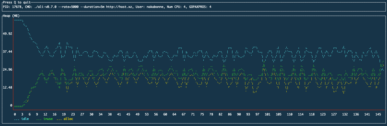
We can see that the addition of the time series storage layer solved the problem of heap usage increasing over time.
tstorage’s drawbacks
tstorage is very simple, so there are still some things that it is not powerful enough for.
For instance, if a single disk partition has a large number of different metrics, there is a problem of the heap becoming overwhelmed. As mentioned earlier, the data itself is mapped in kernel space, so increasing the amount of data is fine. However, all the metadata for the index is on the heap. Because metadata exists for each metric, the number of metadata per partition increases as the number of metrics increases, and the increase in heap usage goes up linearly.
Bottom line:
I feel like time series data is a good subject for implementing a storage engine for the first time because the problems to be handled are simple and can be designed in a straightforward manner.
This post covered the implementation points in an abstract way, but I hope you will have a look at the source code if you are interested.
If you have any questions or feedback, or found out mistakes, it would be great if you could contact me in any way you like.
References
- https://misfra.me/state-of-the-state-part-iii
- https://fabxc.org/tsdb
- https://questdb.io/blog/2020/11/26/why-timeseries-data
- https://questdb.io/blog/2021/05/10/questdb-release-6-0-tsbs-benchmark
- http://www.vldb.org/pvldb/vol8/p1816-teller.pdf
- https://blog.timescale.com/blog/time-series-compression-algorithms-explained